Discussion

Adjustments to fish concentration based on lipid and/or length are necessary to accurately interpret temporal trends in PCB concentration in fish tissue. We initially hoped that modeling on the log-log scale would untangle the time-lipid and time-length interactions. However, this was not generally the case (Table 1). Although each site-species combination varied in the terms that were found to be significant, we felt justified in using the same linear model for each species, regardless of the site. We were not interested in interpreting this linear model and so the significance of any given term was not as important to us as trying to make sure that the adjusted data would be as free as possible from the effects of lipid and length in order to isolate the temporal trend. The adjusted data are our best attempt to show what PCB concentrations would have been if all the fish within a species were identical in length and/or lipid content.

It is important to understand that our predicted PCB concentrations for 2010 are scaled to a historically representative fish. The actual PCB concentrations that are found in future fish will almost certainly continue to vary with lipid content and length.  Although it may be reasonable to say that we are 95% confident that mean PCB concentrations will be within certain limits for fish similar to our representative fish, if the fish are exceptionally different from this representative, we cannot conclude that measured PCB concentrations should be within these limits. It is also important to note that we made predictions only about the mean of the distribution of PCB concentrations for a fish with representative length and lipid content in 2010. The profile likelihood based confidence intervals we generated are not for an individual fish. Individual fish could be expected to have greater variability, though we cannot say how much more based only on our results.

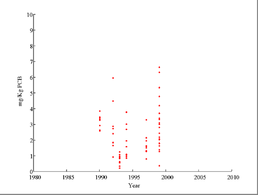
Figure 3: Lake Allegan Carp--Post 1990 Adjusted Data

As noted in the introduction, the mixed-order model asymptotically goes to first order decay as θ goes to 1. For all of the site-species combinations we analyzed, first order decay may be a reasonable model over the study period. It should be noted that in the case of Lake Allegan carp, this approximately first-order model is strongly driven by the exceptionally large sample from 1986 with relatively high levels of PCB. Nearly half of the total data for that site-species combination comes from that year alone. When one looks at post 1990 data only, there appears to be little or no trend (Figure 3).  We suspect that if PCB concentrations start to level off, it will take some time before there are enough years of data to start forcing the fitted mixed order model to differ from first order decay.

Although commonly assumed in the analysis of this type of data, lognormal error does not appear to be a statistically justifiable assumption for two of the four site-species combinations we analyzed. The carp data at both sites were significantly different from lognormal.  The normal probability plot (Figure 2) for Plainwell Impoundment carp data indicates that this significance is probably due primarily to one or two outliers. The normal probability plot for Lake Allegan Carp indicates the deviation from lognormality is not due to the presence of one or two outlying data points. Given the necessity of an error distribution for likelihood based methods and the lack of commonly used alternative error distributions, we continued with the assumption of lognormal error despite the deviations we found. Recognizing the questionable nature of this assumption, we performed the simulation studies to check the robustness of our likelihood-based method and found that, with these data, the method was robust to deviations from lognormal error.

A problem with the two-step procedure using adjusted data is that residuals from the linear model may be dependent. It may also be possible to use likelihood methods to incorporate the dependencies (since they are a function of the design matrix and do not depend on the data values) explicitly. However, the increased amount of computation and coding that would be required to implement this method are probably not justified because the residuals are expected to be nearly independent for sample size much larger than the number of parameters (Graybill, 1976).

There is a second problem with the two-step procedure as we have implemented it; our results do not take into account the variability of parameter estimates in fitting the linear model. The coverage estimates from the third set of simulations indicating actual coverage may be closer to 75% than 95%. This indicates that our intervals are likely to be extremely conservative. This problem needs to be addressed before making any firm claims about what PCB concentrations are likely to be seen in the future. One possible alternative would be to use an a priori adjustment such as a lipid ratio. However, it is not clear that this would accurately account for the effect of lipid and/or length, in general.   Another approach, which we will investigate in future research, is to use a reparameterization of the mixed-order model (Ratkowsky, 1990).  It is hoped that this reparameterization of the mixed-order model will have better convergence properties that would allow a bootstrap approach using Newton-Raphson algorithms to fit the model.