- 2.1
- a) The mean miles per gallon for the 22 two-seater model cars is 25.91
- b) The mean without the Honda Insight is 24.48. The outlier
increases the mean by over 1.4 miles per gallon.
- 2.2
- a) The median miles per gallon for the 22 two-seater model cars is 25.5
The median without the Honda Insight is 25. The outlier only increases the median
by .5 miles per gallon. The median is resistant to outliers whereas
the mean is not.
- 2.3 The median housprice is $163,900 and the mean is
$210,900. Housing prices are skewed to the right, so the mean is
greater than the median.
- 2.5
- a)The five number summary is:
Min = 23040, Q1 = 30387.5, Median = 31975, Q3 = 32710, Max =
33650.
- b) There is some indication of the left skewness. Notice
that the distance from the Median to Q1 is grater than the distance
from the Median to Q3. Likewise the distance from the Median to the
Min is greater than the distance from the Median to the Max.
- 2.6
- a)
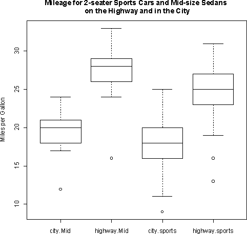
| Data | min | Q1 | median | Q3 | max |
| 2-Seat Highway | 13 | 23 | 25 | 27 | 31 |
| 2-Seat City | 9 | 16 | 18 | 20 | 25 |
| Midsize Highway | 16 | 26 | 28 | 29 | 33 |
| Midsize City | 12 | 18 | 20 | 21 | 24 |
- b)

The mileage in the city seems to generally be much lower than
than mileage on the highway, although there is a small amount of
overlap. The 2-seaters seem to get slightly lower mileage than the
midsize cars, although this difference is small. 2-seaters appear to
have more variability in the mileage than midsize cars.
- 2.9
| Data A | | Data B |
| 1 | 3. | |
| 7 | 4. | |
| | 5. | 3 6 8 |
| 1 | 6. | 6 8 |
| 3 | 7. | 0 7 9 |
| 8 7 1 1 | 8. | 5 8 |
| 3 1 1 | 9. | |
| | 10. | |
| | 11. | |
| | 12. | 5 |
Data A looks like it is left skewed with the majority of the
values between 7 and 9.4. Data B looks more evenly distributed
between 5 and 8 with one outlier at 12.
- 2.15
- a) The mean of the scores is 141.1.
- b) The mean of the scores with the outlier removed is 137.6. The
outlier increases the mean by 3.5.
- 2.17 The median of the scores is 138.5. This is smaller
than the mean. This is the case because of the large outlier
which pulls the mean higher while not impacting the median as
much.
- 2.20

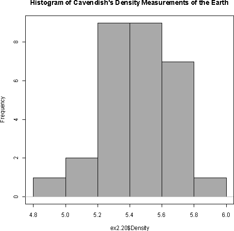
The shape is roughly symmetric with no outliers, so the mean and standard
deviation are probably adequate as summary statistics. The mean is 5.44 and
the standard deviation is 0.22.
- 2.21

| | CA County Populations |
| Min | 1208 |
| Q1 | 46534.25 |
| Median | 159777.5 |
| Q3 | 537352 |
| Max | 9519338 |
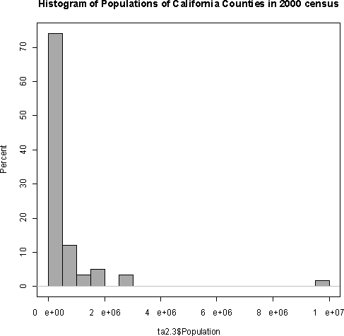
About 75% of the counties have populations less than 500,000, but
there is a long tail on the right side with one very extreme outlier at over
9.5 million people. Based on the histogram, it seems reasonable to divide
the counties into a group with populations less than 350,000, a middle group
with populations between 400,000 and 850,000, and finally a group with
populations over 950,000.
- 2.26 1.5*IQR=1.5*(52.5-30)=33.75 and 110-Q3=110-52.5=57.5, so the
value $110,000 is an outlier by the 1.5IQR rule.
