Chapter 5 Solutions

5.1

a) yhat=31.93426 - 0.30402 x

b) Mean of y (new birds) is 14.23 and the standard deviation is 5.29. Mean of x (percent of returning birds) is 58.23 and the standard deviation is 13.03. The correlation between the two is -0.748.
b = r * s_y/ s_x = -.748 * 5.29/13.03 = -.3037
a = 14.23 - (-.3037)* 58.23 = 31.914

5.3

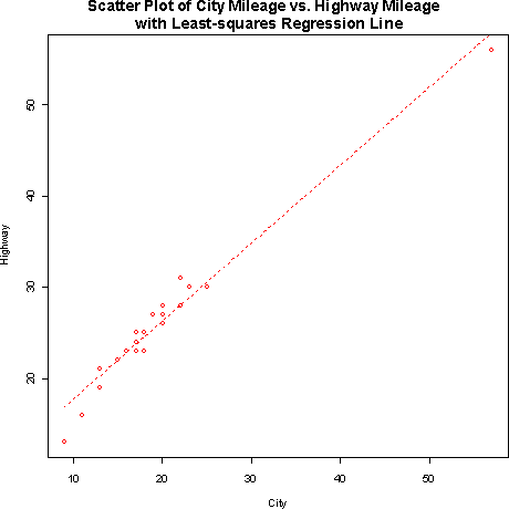
The least squares regression line is yhat = 9.14 + .856 x, where yhat is the predicted highway mileage based upon x, the given city mileage.

b) The slope of the regression line is 0.856. This means that for each additional mile per gallon in the city, car mileage will tend to change by 0.856 miles per gallon on the highway.

c) The predicted highway mileage for a two-seater that is rated at 20 mpg city is approximately 26.259 mpg.

5.5 The mean city mileage is 19.59 mpg and the mean highway mileage is 25.91 mpg. Since the regression line passes through the point (x,y), the predicted highway mileage for a car with 19.59 mpg city, will be 25.91 mpg.

5.8

a) The least-squares regression line of Gessell score on age at first word without Child 19 is: yhat = 109.3 - 1.19 x where yhat is the Gessell score and x is the age at first word (in months).

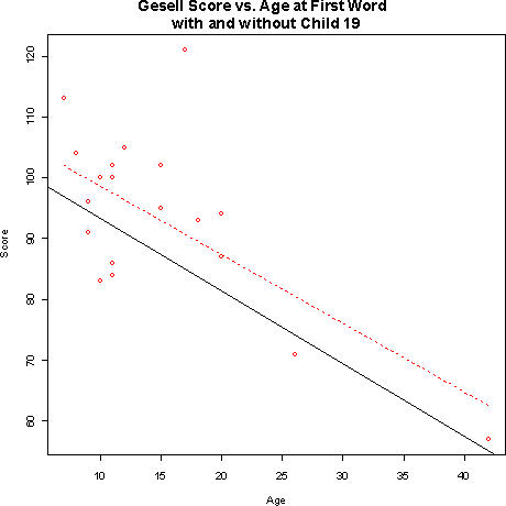
Child 19 does seem to influence the intercept of the regression line, but not the slope. The regression line with Child 19 included (dashed red on the plot) is quite a bit higher than the line with Child 19 not included.

b)The r² changes to .57 without Child 19. This is because Child 19 is an outlier in the y direction. Without it, there is less variation in the y variable, so it is easier for the regression line to 'explain' more of it.

5.9

a, b)

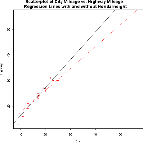
The least squares regression line without the Honda Insight is
yhat = 5.01 + 1.09 x, where yhat is the highway mileage and x is the city mileage.

City MPG	Predicted Highway
City MPG	Regression with Honda Insight	Regression without Honda Insight
10	17.7	15.91
20	26.26	26.81
25	30.54	32.26

5.10

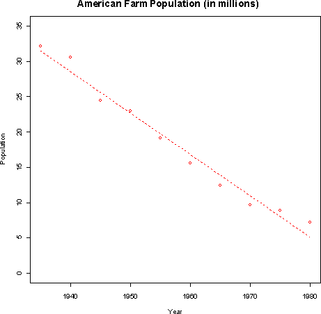
The least-squares regression line is y= 1166.93 - 0.587 x where y is the population in millions and x is the year.

b) According to the regression, the farm population declined by about 587,000 people per year between 1935 and 1980.

c) The predicted population for 1990 is -780,000 people. This is not a reasonable result since population cannot be negative. Regression formulas should genearlly not be used to extrapolate beyond the data.

5.14 Larger hospitals are more likely to have specialized care facilities necessary for treating patients who are very ill. These patients take longer to get well, so this would account for the correlation between hospital size and length of stay.

5.15

a) The correlation between brother's and sister's height is 0.558.

b) The predicted height for Tonya is 64.53.

5.17

a) The slope of the regression line implies that the more TOC there is, the more BOD there will be.

b) The predicted BOD when TOC = 0 is -55.43. This model was probably built using measurements of TOC that were not close to 0. Extrapolation is often inappropriate, as seems to be the case with this model.

5.19

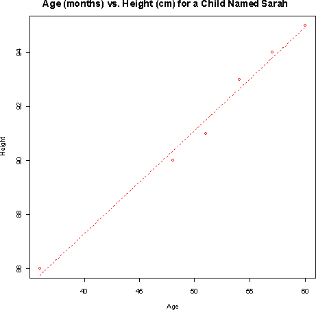
b)The equation of the least-squares regression line is
yhat = 71.95 + 0.383 x where yhat is the height (in cm) and x is the age (in months).

c) The predicted height as 40 months is 87.27 cm. The predicted height at 60 months is 94.93 cm.

d) Sarah's rate of growth is .383 cm per month. The typical rate of growth for girls between the ages of 4 and 5 is 6 cm/12 months = .5 cm per month. Therefore Sarah has grown a little slower than the typical girl.

5.21 Using the regression line from Exercise 5.19, Sarah's predicted height at age 40 (480 months) is 255.79 cm. This is over 100 inches. Linear growth does not persist throughout a human's life.

5.23

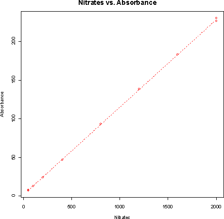
The correlation is 0.9999, so the calibration does not need to be done again.

b) The equation of the least-squares line for predicting absorbence from concentration is y = 1.657 + 0.1133 x. For a specimen with 500 milligrams of nitrates per liter, the predicted absorbence is 58.3. Based on the plot and correlation, this predicted absorbence should be quite accurate.

5.26

a) In each case, the correlation is 0.82, the intercept is approximately 3 and the slope is approximately .5. The predicted y for x = 10 is 8.

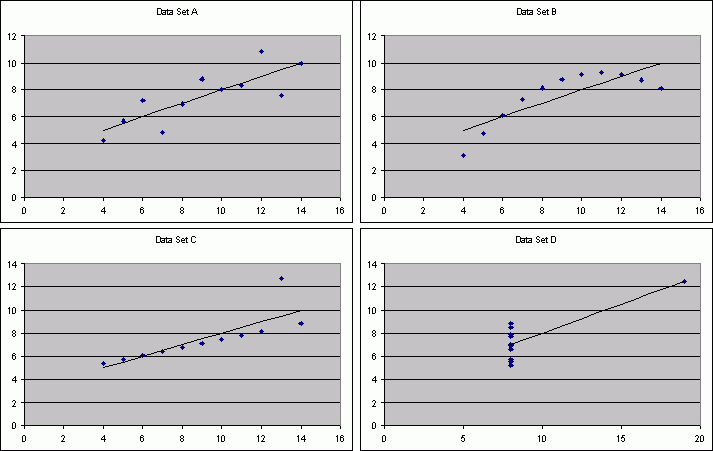
c) For data set A, I would be willing to use the regression to describe the dependence of y on x. There seems to be some variation, about the line, but overall, the relationship seems to be linear. Data set B appears to have a relationship that is non-linear, so the regression does not do a good job of describing the dependence of y on x. Data set C does appear to have a linear relationship with the exception of one point being off the line. This one point causes the regression line to be steeper than it should be to model the relationship for the rest of the data. Data set D does not have enough different x values to say whether or not the regression line is a reasonable description of the dependence of y on x.

5.31 Older kids tend to read better and be taller. The lurking variable of age explains the correlation.

5.41

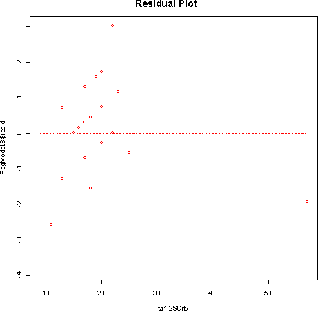
a) The car with the largest positive residual is the Audi TT Roadster (3.03). The car with the largest negative residual is the Lamborghini Murcielago (-3.84).

b) Although the Honda Insight is an outlier, it lies close to the least-squares regression line, so the residual is small.

c) A large positive residual means the car gets better gas mileage on the high than would be expected given its mileage in the city. A large negative residual means the car gets worse highway mileage given its mileage in the city.